10 Function Factories
10.1 Introduction
Function Factory는 functions를 만드는 function이다.
매우 간단한 예를 봐보자.
power1()이라는 function factory를 이용해서, square(), cube()라는 2개의 child 함수들을 만들어보자.
power1 <- function(exp){
  function(x){
    x ^ exp
  }
}

square <- power1(2)
cube <- power1(3)
여기서 square()이랑 cube()는 manufactured functions라고 부른다.
이 용어는 사람과 소통하기 쉽게 하기위해 만들어진거지, R의 관점에서는 다른 함수들과 다를게 없다.
square(3)
## [1] 9
cube(3)
## [1] 27
Function factories를 가능케하는 개별적인 구성요소components들에 대해선 이미 다 배웠다.
-
Section 6.2.3에서, R's first-class functions에 대해 배웠다.
R에서는<-를 이용해서, 오브젝트에 이름을 bind하는 것과 같은 방식으로, 함수function에 이름을 bind할 수 있다. -
Section 7.4.2에서, 함수는 그 함수가 만들어질 때, 함수를 갖고 있는 env를 캡쳐(enclose)한다는 걸 배웠다.
In Section 7.4.2, you learned that a function captures(encloses) the environment / in which it is created. -
Section 7.4.4에서, 함수가 실행될 때마다, 새로운 execution env를 만든다는 것을 배웠다.
이 env는 보통 ephemeral하지만, 여기서는 manufactured function의 enclosing env가 된다.
이 Chapter에서는, 위 3개의 불분명한 조합이 function factory로 이어진다는 것을 배울 것이다.
그리고 visualisation과 statistics에서, function factory의 사용 예제들을 볼 것이다.
3개의 주요 functional programming tools(functional, function factories, function operators)중에서, function factories를 제일 덜 쓴다.
보통, function factories가 전체 코드의 복잡성을 줄여주지는 않는다.
하지만 대신에, 좀 더 소화하기 쉬운 chunks로 복잡성을 줄여준다.
Generally, they don't tend to reduce overall code complexity but instead partition complexity into more easily digested chunks.
또한 Function factories는, 11장에서 배울, 매우 유용한 function operators의 중요한 구성 요소다.
Outline
- Section 10.2에서는, scoping과 env에서 아이디어를 뽑아내서, 어떻게 function factories가 작동하는지를 설명한다.
또한, 어떻게 function factories를 사용해, 함수에 대한 메모리를 implement해서, 호출간에 데이터를 유지할 수 있는지도 살펴본다.
You'll also see how function factories can be used to implement a memory for functions, allowing data to persist across calls. - Section 10.3에서는, ggplot2에서 function factories의 사용예제들을 illustrate할 것.
ggplot2가 user supplied function factories랑 작동하는 것과, function factory를 internally하게 사용하는 것, 총 2가지의 예를 보게 될 것이다. - Section 10.4에서는, statistics의 3가지 challenges를 해결하는데 function factories를 사용한다.
Box-Cox transform을 이해하는 것, Maximum Likelihood 문제를 해결하는 것 그리고 bootstrap resample을 뽑는 것. - Section 10.5에서는, 데이터에서 function families를 빠르게 생성하는데 있어, 어떻게 function factories랑 functionals를 조합할 수 있는지.
Prerequisites
위에 언급한 Section 6.2.3(first-class functions), Section 7.4.2(the function environment) and Section 7.4.4(execution environment)의 내용을 잘 이해하고 있어야함.
Function factories는 base R만 필요하긴 한데, rlang을 이용해서 좀 더 쉽게 들여다보기도 할 것이고, ggplot2와 scales를 이용해서 visualisation에서의 function factories 사용에 대해 탐구해볼 것이다.
library(rlang)
library(ggplot2)
library(scales)
10.2 Factory fundamentals
Function factories가 작동가능한 핵심 아이디어를, 매우 간결하게 표현할 수 있다.
manufactured function의 enclosing env는, function factory의 execution env이다.
간단한 몇 개의 단어로 이 아이디어를 표현할 수 있지만, 이게 무슨 뜻인지 이해하기에는 많은 노력을 필요로 한다.
이 section에서는, interactive exploration과 몇 개의 diagrams를 이용해 이해를 도울 것이다.
10.2.1 Environments
square()과 cube()를 살펴보는 걸로 시작해보자.
square
## function(x){
##     x ^ exp
##   }
## <environment: 0x0000000013e238c8>
cube
## function(x){
##     x ^ exp
##   }
## <bytecode: 0x0000000013cdeff0>
## <environment: 0x0000000013aa9940>
x가 어디서 오는건지는 명확한데, R은 어떻게 exp와 관련되어 있는 값을 찾는거지?
bodies가 똑같기 때문에, manufactured function을 print out해보는건 별 도움이 안된다.
대신에 enclosing env의 내용물이 중요한 factors다.
rlang::env_print()를 이용해서 좀 더 인사이트를 얻을 수 있다.
env_print(square)
## <environment: 0000000013E238C8>
## parent: <environment: global>
## bindings:
##  * exp: <dbl>
env_print(cube)
## <environment: 0000000013AA9940>
## parent: <environment: global>
## bindings:
##  * exp: <dbl>
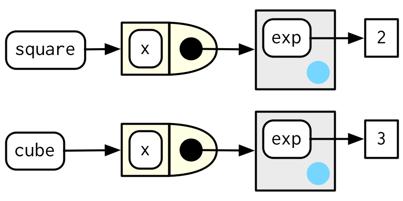
위를 보면, 각각의 manufactured function이 서로 다른 env를 가지고 있다는 걸 보여주는데, 원래 각각은 power1()의 execution env였다.
env들은 같은 parent를 갖고 있는데, power1()의 enclosing env인, global env다.
위를 보면, 2개의 env 다 exp라는 binding을 갖고 있는 것을 볼 수 있는데, 우리는 그 값을 보고 싶다.
이럴 때는 function env를 가져와서 값을 추출하면 된다.
fn_env(square)$env
## NULL
fn_env(cube)$env
## NULL
이게 각 manufactured function이 서로 다르게 작동하는 이유이다.
enclosing env에 있는 names가 서로 다른 값에 bound되어 있다.
10.2.2 Diagram conventions
이 관계를 다이어그램으로도 나타내 볼 수 있다. 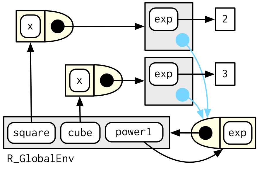
이 다이어그램에는 뭐가 많지만, 몇몇 디테일은 중요하지 않다.
2개의 conventions를 이용해 상당히 단순화할 수 있다.
-
모든 free floating symbol은 global env에 산다.
-
분명한 parent가 없는 env라면, global env로부터 inherit한다.
env에만 집중한 이 다이어그램을 보면, cube()와 square()간의 아무런 직접적인 링크가 없다는걸 볼 수 있다.
왜냐하면 링크는 둘 다 같은 함수의 body를 통해서만 존재하는데, 이 다이어그램에는 존재하지 않는다.
마지막으로, square(10)을 불렀을 때의 execution env를 봐보자.
square(10)
## [1] 100
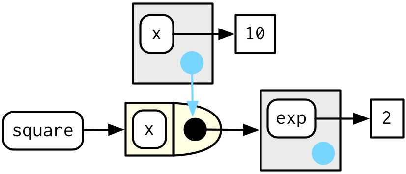
square()이, x ^ exp 를 실행할 때, x는 execution env에서 찾고, exp는 enclosing env에서 찾는다.
10.2.3 Forcing evaluation
power1()에는 lazy evaluation으로 인한 미묘한 버그가 있다.
이 문제를 묘사하는 예를 보자.
x <- 2
square <- power1(x)
x <- 3
그럼 여기서 square(2)를 하면 무슨 값이 나올까? 4겠지?
square(x)
## [1] 27
8이 나온다. 왜냐하면 x는, power1()이 실행될 때 evaluate되는 것이 아니고, square()가 실행될 때 evaluate되기 때문이다.
보통 이런 문제는, function factory를 calling하는 거랑 manufactured function을 calling하는 것 사이에 binding이 바뀔 때, 발생한다.
이러한 일은 잘 일어나지 않는데, 일어나면 머리 아픈 버그가 발생한다.
이 문제를 force()를 사용해서 evaluation을 forcing할 수 있다.
power2 <- function(exp){
  force(exp)
  function(x){
    x ^ exp
  }
}

x <- 2
square <- power2(x)
x <- 3
square(2)
## [1] 4
이렇게 하면 문제가 없는걸 볼 수 있음.
function factory를 만들 때, argument가 manufactured function에 의해서만 사용되는거라면, force()를 이용해서 확실하게 evaluate해라.
10.2.4 Stateful functions
Function factories는 함수 호출function invocation간에 state를 유지할 수 있도록 해준다. 이건 Section 6.4.3의 fresh start principle때문에 원래는 힘든 것이다.
이걸 가능케하는 2가지 것들이 있다.
-
manufactured function의 enclosing env는 unique하고 constant하다.
-
R은 enclosing env에 있는 bindings를 수정해주는,
<<-라는 특별한 할당 연산자special assignment operator가 있다.
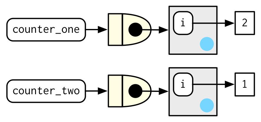
이 아이디어들을 종합해서, 몇 번이나 호출되었는지를 기록하는 함수를 만들어보자.
new_counter <- function() {
  i <- 0

  function() {
    i <<- i + 1
    i
  }
}

counter_one <- new_counter()
counter_two <- new_counter()
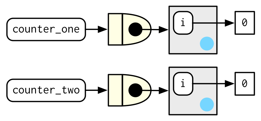
manufactured function이 실행될 때, enclosing env에 있는 i를 i <<- i + 1이 수정한다.
각 manufactured function은 독립적인 enclosing env를 가지고 있기 때문에, 독립적인 counts를 갖는다.
counter_one()
## [1] 1
counter_two()
## [1] 1
counter_one()
## [1] 2
상태를 저장하는 함수, stateful functions는 적당히 사용하는게 좋다.
함수가 여러 변수의 state를 managing하는 단계가 되면, 14장의 주제인 R6로 바꾸는게 좋다.
As soon as your function starts managing the state of multiple variables, it's better to switch to R6, the topic of Chapter 14.
10.2.5 Garbage collection
대부분의 함수와 같이, garbage collector로 하여금, 함수 안에 만들어지는 용량 큰 temporary object들을 clean up하도록 기대할 수 있다.
그런데, manufactured function의 경우에는 execution env에 매달려있기 때문에, rm()을 사용해서 용량 큰 object들을 명백하게 unbind해줘야 한다.
아래의 예에서, g1()과 g2()간의 용량을 비교해보자.
f1 <- function(n) {
  x <- runif(n)
  m <- mean(x)
  function() m
}

g1 <- f1(1e6)
lobstr::obj_size(g1)
## 8,013,136 B
f2 <- function(n) {
  x <- runif(n)
  m <- mean(x)
  rm(x)
  function() m
}

g2 <- f2(1e6)
lobstr::obj_size(g2)
## 12,976 B
10.2.6 Exercises
force()의 정의는 단순하다:
force
## function (x)
## x
## <bytecode: 0x0000000012db2750>
## <environment: namespace:base>
force(x)가 x보다 나은 이유는 무엇일까?
-
base R은 2개의 function factories,
approxfun()과ecdf()를 갖고 있다. documentation을 읽고, 이 함수들이 뭘하고 무엇을 return하는지 알아내라. ?approxfun -
i라는 index를 argument를 받는 함수pick()을 만들어라. argumentx를i로 subset한 함수를 return해야함.
그러니까,pick(1)(x)은,x[[1]]와 같은 것이어야하고,lapply(mtcars, pick(5))은,lapply(mtcars, function(x) x[[5]])와 같은 것이어야 한다.
pick <- function(){
- numeric vector의 ith central moment를 계산하는 함수를 만드는 함수를 만들어라.
다음의 코드를 실행해봄으로써 잘 만들어졌는지 테스트를 해볼 수 있다.
10.3 Graphical factories
ggplot2에서 몇몇 예를 보면서, 유용한 function factories에 대해 탐구해보자
10.3.1 Labelling
scales 패키지의 목표 중 하나는, ggplot2에서 라벨label을 customise하기 쉽게 만들어주는 것이다.
축들axes과 범례legends의 세부 내용을 컨트롤할 수 있는 많은 함수들을 공급provide해준다.
포맷 함수들formatter functions는, 축 브레이크axis breaks의 외형을 컨트롤할 수 있는 유용한 class of functions다.
첫 눈에 보기엔 조금 이상하다: number를 형식화format하기 위해 호출하는데, function을 return하니깐.
y <- c(12345, 123456, 1234567)
comma_format()(y)
## [1] "12,345" "123,456" "1,234,567"
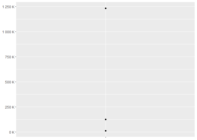
number_format(scale = 1e-3, suffix = " K")(y)
## [1] "12 K" "123 K" "1 235 K"
즉, 기본 인터페이스는 function factory다.
언뜻 보기엔, 조금의 이득을 위해서 엄청 복잡하기만 해진 것 같다.
하지만 ggplot2의 스케일과 좋은 상호작용interaction을 하는게, label argument에서 함수를 받아주기 때문.
df <- data.frame(x = 1, y = y)
par(mfrow = c(2, 2))
core <- ggplot(df, aes(x, y)) +
  geom_point() +
  scale_x_continuous(breaks = 1, labels = NULL) +
  labs(x = NULL, y = NULL)

core
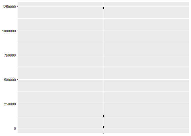
core + scale_y_continuous(
  labels = comma_format()
)

core + scale_y_continuous(
  labels = number_format(scale = 1e-3, suffix = " K")
)
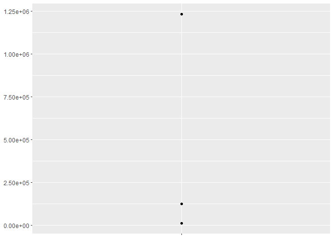
core + scale_y_continuous(
  labels = scientific_format()
)
10.3.2 Histogram bins
geom_histogram()의 binwidth argument도 함수가 될 수 있다는게 잘 알려진 특성feature이다.
이건 특히나 유용한게, 각 그룹에 따라 function이 execute될 수 있기 때문에, 다른 측면facets에 따라 다른 binwidth를 가질 수 있다는 것.
이 아이디어를 illustrate, 고정된 binwidth가 유용하지 않은 예를 만들어 보이겠다.
sd <- c(1, 5, 15)
n <- 100

df <- data.frame(x = rnorm(3 * n, sd = sd), sd = rep(sd, n))

ggplot(df, aes(x)) +
  geom_histogram(binwidth = 2) +
  facet_wrap(~ sd, scales = "free_x") +
  labs(x = NULL)
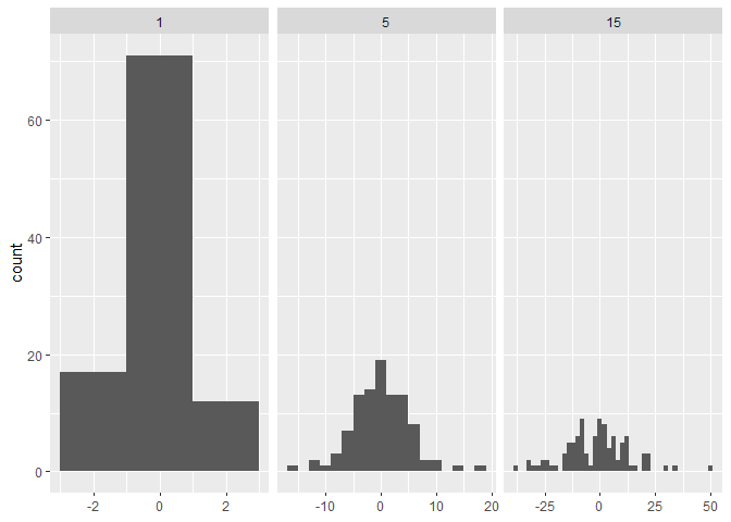
여기서 각 facet는 같은 수의 observations를 갖고 있는데, 여기서 variability가 매우 다르다.
binwidths가 달라지게 해서,